Analytic result + secondary evidence + registered protocol
How many Lighthouse runs prove a change?
“We ran it five times and the score went up two points.” That sentence drives sprint reviews, agency invoices and CI gates — and most of the time it isn't evidence. Lighthouse is noisy enough that a small before/after change can be pure run-to-run variance. Median-of-five gives you a stable estimate; it does not give you the statistical power to prove a small improvement is real. Here's the framework that does — with the numbers, a calculator, and the protocol to settle it at scale.
What's settled here, and what isn't
This article delivers three things and is careful to keep them apart. (1) A completed analytic result — the confidence-interval and power tables that convert a run-level standard deviation into the runs you need; these are mathematics, not measurement. (2) Secondary empirical evidence — real repeated-run Lighthouse data from a published study, showing the variance is large and site-specific. (3) A registered protocol for the primary study we have not yet run (a 200-site × 50-run variance census). No empirical variance number is invented; the analytic tables are exact evaluations of the stated known-σ normal-approximation formula, and the census is specified so it can be executed and audited.
The claim everyone makes — and why it's usually unproven
The advice to run Lighthouse multiple times and aggregate is correct and well-founded. Google's own variability guidance lists the sources of run-to-run noise — network, CPU contention, layout non-determinism, A/B and personalisation — and recommends aggregating runs. The closest academic study, Heričko, Šumak & Brdnik (2021), reaches the same operational rule: single runs are unrepresentative, and five consecutive runs aggregated by the median reduce variability greatly in reasonable time. That is where “median of 5” comes from, and for its purpose — a stable snapshot of one page — it's good guidance.
It is worth being precise about how much that study can carry, because it is routinely cited as proof that five runs are enough. Its test was Mood's median test comparing the realised N=5, N=10 and N=100 groups per site; most p-values exceeded 0.05, and the authors concluded five runs were sufficient relative to ten and a hundred. But failing to reject equal medians is not evidence of equivalence — with one five-run group per site, non-rejection is exactly what low power produces, and no equivalence margin was declared. The design also cannot speak to the question that matters here: it observed one median-of-5 per site, so it never estimated how much a median-of-5 varies from batch to batch. Read it as strong evidence that single runs are unrepresentative and that aggregation helps — not as a precision guarantee.
The trouble is that the same heuristic gets quietly promoted to a job it was never validated for: proving that a change moved the score. Stabilising an estimate and detecting a small difference are different statistical problems. The first asks “where does this page sit?”; the second asks “is this 2-point gap bigger than the noise?” — and the answer to the second depends entirely on how much the runs scatter relative to the change you're claiming.
The variance is real, large, and stubbornly site-specific
Before any statistics, look at what repeated runs actually do. Heričko et al. ran each of ten production sites 1, 5, 10 and 100 times. Aggregation does pull the median in — but the underlying spread is wide for some sites and tiny for others, and it does not vanish even at 100 runs:
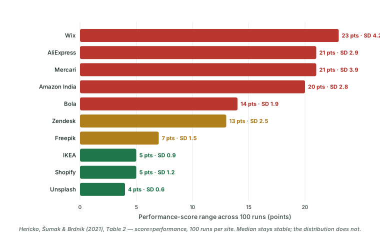
Two things explain why the score is so jumpy. First, its composition: the score is a weighted blend of metrics with very different noise behaviour, and the blend has changed. Today (Lighthouse 10+) Total Blocking Time carries 30%, LCP and CLS 25% each; the runs charted above were collected on Lighthouse 7.3.0, whose score weighted FCP 15%, Speed Index 15%, LCP 25%, Time to Interactive 15%, TBT 25% and CLS 5%. So the figures above are evidence that the score is noisy, but they were produced by a different instrument: today's weights do not explain that particular variance, and today's variance cannot be read off it either — CLS went from 5% to 25% of the score, and Time to Interactive left the score entirely. Either way TBT, which depends on exactly how main-thread long tasks get scheduled, is among the most timing-sensitive inputs, and it weighs more now than it did then. Second, throttling: PageSpeed Insights and default Lighthouse use simulated (Lantern) throttling, whose modelled timings react differently to noise than applied throttling. The upshot is that a “run-level σ” of 2 points on one site can be 7+ on another in the same lab — which is why a borrowed variance number is unsafe and a pilot is mandatory.
The right question is power, not repetition
Treat a before/after comparison as what it is: a two-sample test on noisy measurements. To detect a true difference δ in the score, with run-level standard deviation σ, at two-sided significance α and power 1−β, the runs per condition follow the standard sample-size formula:
n  ≥  2 · (z₁₋α/₂ + z_power)² · σ² / δ²        independent, equal n per condition

at α = 0.05 and power = 0.80:   n  ≈  15.7 · σ² / δ²

paired runs (alternated before/after):  drop the factor of 2, use σ of the paired differences
The σ²/δ² term is the whole story. Runs scale with the square of the
noise-to-signal ratio, so halving the change you want to detect quadruples the runs you need.
That is why “a few more runs” never rescues a small claim — and why the median-of-5 default silently
fails the moment the effect you're chasing is small relative to the spread.
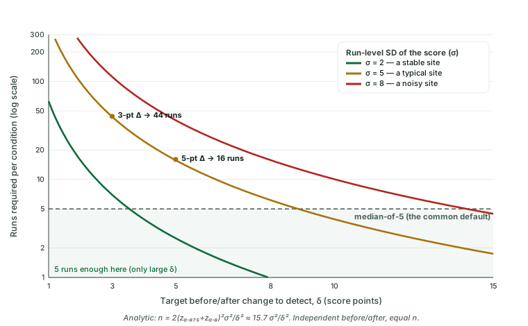
| Detect δ | σ = 2 | σ = 5 | σ = 8 |
|---|---|---|---|
| 10 points | 1 | 4 | 11 |
| 5 points | 3 | 16 | 41 |
| 3 points | 7 | 44 | 112 |
| 1 point | 63 | 393 | 1,005 |
What median-of-5 can and can't prove
Read the same physics the other way: fix the runs and ask how small a change they can resolve. Two different numbers get called “the smallest change you can prove,” and conflating them is the most common mistake in this whole area:
- The observed significance threshold —
z₁₋α/₂ · σ · √(2/n)— is how big a measured difference must be for the test to reject zero. At n = 5 and σ = 5 that is 6.2 points: a measured 7-point gap really does come out significant (p ≈ 0.027). - The minimum detectable effect (MDE) —
(z₁₋α/₂ + z_power) · σ · √(2/n)— is the size a true effect must have before this design is likely (here 80%) to detect it. At n = 5 and σ = 5 that is 8.9 points for run means.
The MDE is the honest planning number, because a design that only rejects zero 80% of the time when
the effect is real will stay silent one run in five. But note what it is not: it is not a floor below
which a result cannot be significant. Both shrink only as 1/√n — brutal diminishing
returns. Here is what each run budget buys in the illustrative σ = 5 scenario:
And “median-of-5” is not the same estimator as “mean-of-5”
Everything above — and the n ≈ 15.7 σ²/δ² table — is derived for the difference of
two means. The prevailing practice aggregates by the median, and a median is a
less efficient estimator of location: under normality its sampling variance is about
π/2 ≈ 1.57× the mean's, because median precision depends on the density at the
centre rather than on σ alone.
So the mean-based 8.9 does not transfer to medians. Simulating the difference of two medians of five normal draws directly (σ = 5, two-sided α = 0.05) puts the 80%-power point at ≈ 10.6 points — and at 8.9 points the median-of-5 design has only about 65% power. Read the tables as mean-based planning numbers; if you aggregate by the median, budget roughly 1.5× the runs, or state the estimator and simulate it for your own pilot distribution — Lighthouse scores are bounded and can be skewed, so the normal approximation is a starting point, not the last word.
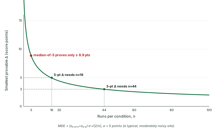
So median-of-5 isn't wrong — it's a screening tool. It will reliably flag a page that fell off a cliff. It cannot, and was never meant to, certify that your CSS refactor bought 3 points. For that you need either many more runs, a paired design that cancels shared drift, or the honesty to report “within noise.” This is the same lesson the systems-benchmarking literature settled long ago: Mytkowicz et al. showed you can “produce wrong data without doing anything obviously wrong,” and Kalibera & Jones formalised how many repetitions rigorous benchmarking actually requires. Web performance is not exempt.
Put your own numbers in
The tables above assume round numbers. Your site has its own spread, and your claim has its own threshold. The companion calculator turns a pilot-measured σ and a target δ into the runs you need — and, for any candidate run count, the smallest change you could honestly claim and the confidence interval you'd report.
Lighthouse required-runs calculator
Enter your run-level SD, the change you want to prove, and your confidence and power. It returns the required runs per condition, a precision sweep, and a clear red/green read on whether your planned run budget can actually support the claim.
The protocol to settle σ empirically
The analytic tables need one input the literature only sketches: the real distribution of run-level σ across the web, by site class and setup. The registered primary study fills that gap, and ships its data schema pre-frozen so results can't be fished:
A 200-site × 50-run census
200 sites stratified by score band, framework, third-party intensity and content class, each run 50× per condition on a pinned single-tenant runner — enough to estimate per-site σ precisely and to map how σ varies across the web.
Fixed environment, recorded to the byte
One Lighthouse version, Chrome build, throttling mode, device profile and cache policy, with container digest, CPU model and governor, and cgroup quota logged per run (the raw-observation schema is in the pack). Variance you don't control, you record.
Per-metric, not just score
σ for FCP, LCP, SI, TBT and CLS separately — the census measures, rather than assumes, how much of the score's noise is TBT's — and a fix that targets LCP should be judged on LCP, not on a composite in which TBT carries the largest weight.
Bootstrap, not just the normal approximation
The closed-form n assumes approximate normality of the mean; the study reports bootstrap confidence intervals on the median-of-n as well, since medians are what practitioners actually quote.
A published claim standard
The deliverable is a per-site-class table of “runs needed to defensibly claim a δ-point change,” turning the calculator's general formula into concrete, citable guidance.
A defensible before/after claim
Pulling it together, a Lighthouse before/after claim is decision-grade only when it clears a short bar. Anything less is a screening signal, and should be labelled as one:
- Pre-register δ. Decide the smallest change worth claiming before measuring — not after seeing the result.
- Pilot your σ. Estimate run-level spread in your exact setup; don't borrow a number.
- Hit the required n. Use
n ≈ 15.7 σ²/δ²(or the calculator); median-of-5 only qualifies when δ is large relative to σ. - Pair or block. Alternate before/after runs to cancel shared drift; it can cut the runs needed substantially.
- Report the interval. Quote a confidence interval on the difference, not two point medians. “+3 ± 6” is an honest non-result; “+3” alone is misleading.
- Freeze the environment. Same version, throttling, device and cache — and judge a metric-targeted fix on that metric, not the composite.
Limitations
σ is an input, not yet a measured distribution
The tables are exact arithmetic for a given σ under the stated model; the spread of σ across the real web is what the registered census exists to supply. Until then, use a pilot — and treat σ = 5 as an illustrative high-noise scenario rather than a typical value. The only per-site spreads we can point at are the ten in Heričko et al.'s 100-run groups: 0.6 to 4.2 points, mean 2.24 — desktop, ten sites, Lighthouse 7.3.0, so not a population estimate either, but nothing in it supports calling 5 typical.
Normal-approximation closed form
The
nformula assumes approximate normality of the aggregated mean and a known σ. For small n and skewed metrics (TBT, CLS), prefer the bootstrap; the secondary-evidence ranges hint the score is not always symmetric.Score vs metrics
This focuses on the 0–100 performance score for continuity with the median-of-5 advice. The same machinery applies per metric, with different σ — often the more useful unit.
Lab, not field
This is about controlled lab repeatability, not CrUX field data. A change that's lab-significant still has to show up for real users — a separate question we treat in our other studies.
Data, code & sources
Published under CC BY 4.0: the digitised secondary evidence, the analytic CI-multiplier and minimum-detectable-effect tables, and the pre-frozen raw-observation schema for the census. Every analytic number is reproducible from the formulas above.
Key sources
- Heričko, T., Šumak, B. & Brdnik, S. (2021). Towards Representative Web Performance Measurements with Google Lighthouse, StuCoSReC 2021 — the repeated-run data (Table 2) and the median-of-5 finding.
- Google / Chrome. Lighthouse performance scoring (metric weights: TBT 30%, LCP 25%, CLS 25%, FCP 10%, SI 10%) & Lighthouse variability (sources of noise; aggregate runs).
- DebugBear. Reducing variability in web performance metrics — independent repeated-run evidence.
- Mytkowicz, T. et al. (2009). Producing wrong data without doing anything obviously wrong!, ASPLOS — measurement bias in benchmarking.
- Kalibera, T. & Jones, R. (2013). Rigorous benchmarking in reasonable time, ISMM — how many repetitions rigorous measurement needs.
Cite this study
PageSpeedAudit Research (2026). How many Lighthouse runs prove a change?
A confidence-interval and statistical-power framework for before/after
performance-score claims.
https://pagespeedaudit.com/research/how-many-lighthouse-runs-prove-a-change

@misc{pagespeedaudit2026lighthousepower,
  title  = {How many Lighthouse runs prove a change? A confidence-interval
            and statistical-power framework for before/after claims},
  author = {{PageSpeedAudit Research}},
  year   = {2026},
  url    = {https://pagespeedaudit.com/research/how-many-lighthouse-runs-prove-a-change},
  note   = {Analytic tables + secondary evidence + registered protocol, CC BY 4.0}
}
Want a before/after you can actually defend?
A PageSpeedAudit report reports effects with their uncertainty, not a lone point score — so a “+3” comes with the interval that tells you whether it's real. Try the free required-runs calculator, and see our sister study “Do Lighthouse's promised savings materialize?” for whether the predicted milliseconds even show up.